72% of engineering mistakes come from missed equations or wrong units. A reliable reference can save hours and prevent costly rework.
We created this ultimate mechanical engineering formula sheet. It’s a compact, authoritative guide for engineers, students, and instructors.
The sheet covers key equations in Engineering Mechanics, Strength of Materials, Fluid Mechanics, and more. It includes Thermodynamics, Heat Transfer, Machine Design, Vibrations, manufacturing, and control topics.
Each section has formula boxes with units, short explanations, typical assumptions, and diagram guidance. This helps you use equations quickly and confidently.
We made the content easy to navigate. You’ll find a downloadable PDF cheat sheet and printable reference at the end of the article for offline use.
Mechanical Engineering Formula Sheet – All Key Equations in One Place

We made a handy guide for everyday formulas engineers use. This sheet organizes equations by topic. It includes units, assumptions, and examples for quick use.
What this sheet includes
It covers statics, dynamics, stress, and strain. Also, fluid relations, thermodynamics, heat transfer, and machine design. Plus, manufacturing metrics, vibrations, controls, and instrumentation.
Each formula shows units, typical ranges, and a simple example. It’s a practical reference for design checks and analysis.
How to use the formulas effectively
Always use SI units. Sketch diagrams and state assumptions first. This helps in solving equations.
Check dimensions and use property tables for data. Apply empirical correlations for design based on experiments. Use exact solutions for well-defined conditions.
Define the system, choose equations, reduce with assumptions, solve, and validate. This makes the guide useful for projects and exams.
Downloadable PDF cheat sheet link
Get a two-page cheat sheet for quick reference. Or a longer PDF with derivations, examples, and tables. The full PDF is a detailed handbook for study and design.
The short cheat sheet gives you the most important formulas at a glance. The full PDF helps with step-by-step solutions and examples from real engineering tasks.
Engineering Mechanics: Statics and Dynamics Essential Equations

We collect key engineering mechanics equations for solving forces, moments, and motion. This guide breaks down into planar and spatial cases. It also distinguishes between particle and rigid-body models for easy use.
Equilibrium equations for rigid bodies
For a rigid body at rest or moving steadily, use sum rules: ΣF = 0 and ΣM = 0 in vector form. In two dimensions, apply ΣFx = 0, ΣFy = 0, ΣM = 0. Use SI units: N for forces and N·m for moments.
Choose a consistent sign convention and a moment center to simplify calculations. For three-dimensional problems, use the vector moment r × F to compute torques. Include all moment components when assembling statics and dynamics formulas.
Free-body diagrams and reaction forces
Isolate bodies and replace supports with reaction components. For beams and trusses, mark pinned and roller supports. Then, write equilibrium for forces and moments.
Typical reaction equations exist for simply supported and cantilever beams with point loads and uniform distributed loads. When solving statically determinate structures, count unknowns and independent equilibrium equations. Free-body diagrams are the first step when applying key mechanical engineering formulas.
Kinematics of particles and rigid bodies
Kinematic relations define position, velocity, and acceleration: s, v = ds/dt, a = dv/dt for particles. For rotation, use θ, ω = dθ/dt, α = dω/dt. Units include meters, m/s, m/s² and radians, rad/s, rad/s².
Apply relative motion equations for connected bodies and use rigid-body kinematics for points fixed in a rotating body. These statics and dynamics formulas help link geometry with motion before applying forces.
Newton’s laws for dynamics
For particles, apply F = ma. For rigid bodies, use ΣM = Iα about an appropriate axis. Use linear and angular momentum principles when impulse or conservation is relevant.
Complement force methods with energy relations: W = ΔKE and ∑Work = Δ(½mv² + ½Iω²). Energy-based approaches often simplify problems with variable forces. They can reduce algebra when paired with other engineering equations.
Practical tips: Start with a clear free-body diagram, pick convenient axes, check units, and consider energy methods when forces vary with position. These steps keep key mechanical engineering formulas and statics and dynamics formulas organized for reliable results.
Strength of Materials: Core Formulas for Stress and Strain

This guide is a quick reference for engineers. It covers formulas for stress and strain in daily work. You’ll learn to size shafts, beams, and fasteners confidently.
Axial relationships
Axial normal stress is σ = F/A. Axial strain is ε = ΔL/L. Hooke’s law links them: σ = Eε. For thermal effects, use ε_th = αΔT.
Steel’s elastic modulus is about 200 GPa. These formulas are key in mechanical engineering.
Torsion of circular shafts
Shear stress in a circular shaft is τ = Tρ/J. Maximum shear stress is at ρ = outer radius. Angle of twist is θ = TL/(GJ).
The polar moment for a solid shaft is J = πd4/32. Use N·m and Pa for units. Check shear modulus G before design.
Bending and flexure
Bending stress is σ = My/I. Use these formulas for midspan stresses and support reactions.
Combined loading and principal stresses
For multisource loading, use transformation equations. Compute principal stresses by σ1,2 = (σx+σy)/2 ± sqrt[((σx-σy)/2)2 + τxy2].
Von Mises equivalent stress is σv = sqrt[σx2 – σxσy + σy2 + 3τxy2]. This formula assesses ductile failure.
Practical notes
Include stress concentration factors for notches and holes. Choose factors of safety based on material data. Compare yield criteria like Tresca and von Mises.
Use this sheet for quick reference to stress and strain equations. It’s part of a complete toolkit for mechanical engineering.
Fluid Mechanics: Key Equations and Flow Relations
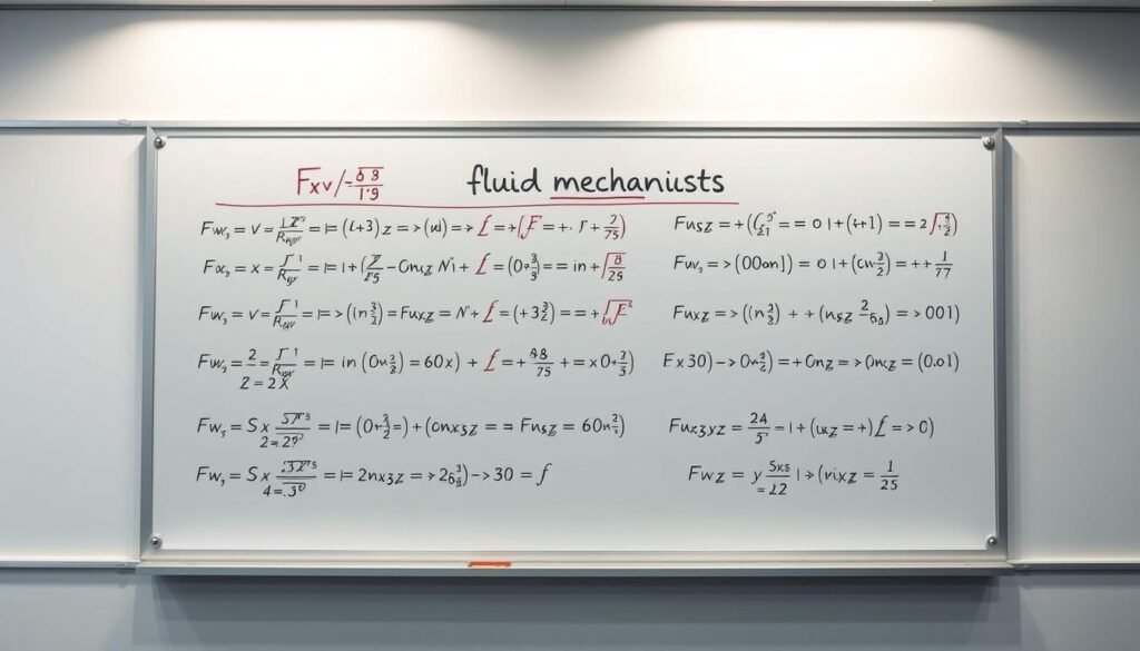
We present the core relations you will reach for when solving flow problems. This compact guide blends fundamental theory with practical cues so we can choose the right model quickly.
Continuity and volumetric flow rate
The continuity equation enforces mass conservation: ρ1A1V1 = ρ2A2V2 for compressible flows. For incompressible liquids, it simplifies to A1V1 = A2V2. This gives us volumetric flow in m^3/s. Use the steady form for time-invariant cases and the unsteady form when density or area change with time. Open-channel analogs follow the same mass-balance logic but use cross-sectional area and depth variations.
Bernoulli and energy conservation
The Bernoulli equation links pressure, kinetic, and potential heads along a streamline: p/ρg + V^2/2g + z = constant for inviscid, incompressible, steady flow. For real flows, add head loss hL: p/γ + V^2/2g + z + hL = constant. Express terms in Pascals or in meters of head depending on the calculation. Use the Bernoulli equation as an energy check in piping and open-channel problems.
Navier–Stokes overview and simplifications
The Navier–Stokes momentum balance describes Newtonian fluid motion with viscous stresses, body forces, and pressure gradients. Full solutions require numerical methods for most engineering geometries. We often apply simplified forms: Euler equations for inviscid flow, boundary-layer equations near walls, creeping flow for very low Reynolds number, and potential flow when rotation of fluid elements is negligible. Choose the simplification that preserves the dominant physics.
Laminar vs turbulent flow and Reynolds number
Re = ρVD/μ defines the flow regime: low Re yields laminar profiles, high Re yields turbulence. In circular pipes, transition occurs near Re ≈ 2300. Laminar flow has parabolic velocity profiles; turbulent flow has fuller profiles and enhanced mixing. For head loss, use Darcy–Weisbach: hL = f (L/D) V^2/2g. Friction factor f comes from exact solutions in laminar flow or from empirical fits and the Moody chart for turbulent flow; Colebrook gives an implicit relation for rough pipes.
Practical correlations and tips
When field data dominate, use empirical formulas such as Hazen–Williams for water mains. For short pipes or fittings, apply localized loss coefficients. Sketch streamlines, velocity profiles, and a pipe cross-section with boundary layer when documenting assumptions. Keep a mechanical engineering reference guide or cheat sheet at hand to speed selection of formulas during design work.
| Relation | Form | Typical Use |
|---|---|---|
| Continuity equation | A1V1 = A2V2 (incompressible) | Pipe sizing, flow splits, mass balance |
| Bernoulli equation | p/ρg + V^2/2g + z + hL = constant | Energy heads, pump and turbine work estimates |
| Navier–Stokes | ρ(∂V/∂t + V·∇V) = −∇p + μ∇^2V + ρg | Detailed CFD, complex viscous flows |
| Reynolds number | Re = ρVD/μ | Predict laminar vs turbulent, select friction correlations |
| Darcy–Weisbach | hL = f (L/D) V^2/2g | Head loss in pipes, pressure drop estimates |
We frame these essential engineering equations inside a compact mechanical engineering reference guide to help with quick checks and rigorous calculations. Use the continuity equation and Bernoulli equation for first-order designs and reserve Navier–Stokes and CFD for detailed validation.
Thermodynamics: Fundamental Laws and Property Relations

We have a quick guide to thermodynamics equations and useful relations for energy systems. It’s perfect for any mechanical engineering formula sheet. It explains key concepts and when to use different methods.
First and second law equations for closed and open systems
For closed systems, use ΔE = Q – W. This equation covers internal, kinetic, and potential energy changes. For open systems, the steady-flow energy equation is ṁ(h + V^2/2 + gz)_in + Q̇ – Ẇ = ṁ(h + V^2/2 + gz)_out.
The second law tells us ΔS_total ≥ 0. It also helps us understand reversible versus irreversible processes with the Clausius inequality.
Ideal gas relationships and real gas corrections
The ideal gas law is PV = nRT or p = ρRT. Use cp and cv for specific-heat relations. For non-ideal gases, consider Z or virial coefficients.
For precise calculations, check NIST property data or engineering gas tables. They offer more accurate results than the ideal gas law.
Thermodynamic cycles: Carnot, Otto, Diesel formulations
Important cycle metrics include Carnot efficiency η = 1 – Tc/Th. Ideal Otto efficiency is η = 1 – r^(1-γ) with r as compression ratio and γ the heat-capacity ratio. Diesel and Brayton cycles have similar expressions for work and heat.
Use mean effective pressure to link cycle work to engine displacement. This is crucial for engine design.
Property tables, specific heats, and state relations
Steam tables and refrigerant charts are great for quick conversions. Use temperature-dependent cp values or ideal-gas polynomials for accurate heat calculations. Always keep units consistent to avoid errors.
Practical notes and tools
For complex mixtures or flows, EES, REFPROP, or Aspen are good tools. Sketch P–V and T–s diagrams to understand cycles better. Keep a single-page mechanical engineering formula sheet handy for quick reference.
Heat Transfer: Conduction, Convection, and Radiation Formulas
We offer a quick look at key heat transfer formulas and tips for thermal design. Our aim is to make these formulas easy to use in calculations and quick checks. This section connects theory to practice with clear equations and guidelines.
Fourier’s law explains steady one-dimensional conduction: q = -kA dT/dx. Use thermal resistance R_th = L/(kA) for layered systems. Keep units right: k in W/m·K, q in W. These formulas help us turn gradients into heat rates for different shapes.
Convective heat transfer is q = hAΔT, with h in W/m^2·K. Nusselt number correlations give h from flow conditions: Nu = hL/k. Use Dittus-Boelter for turbulent internal flow and Churchill–Bernstein for external flows. These correlations link fluid dynamics to surface heat flux.
Radiation emission from a surface follows the Stefan–Boltzmann relation q = εσAT^4, with σ = 5.670374×10^−8 W/m^2·K^4. For net exchange between surfaces, use view factors and radiosity. Be careful with emissivity: gray-body assumptions are common, but temperature-dependent emissivity can affect results.
Transient heat conduction often starts with the lumped capacitance model when Biot number Bi = hL_c/k is below 0.1. Then T(t) = T∞ + (T0 – T∞) e^(-hA/(ρVc) t) models the exponential approach to ambient. For Bi > 0.1, use series solutions or numerical methods and consult Heisler charts for common geometries.
Practical diagram suggestions include: a temperature profile through a slab, a fin schematic showing conduction to convection, and an RC analogy for lumped systems. Remember that material properties vary with temperature and that unit consistency prevents subtle errors when applying heat transfer formulas in design work.
| Mode | Primary Equation | Key Dimensionless | When to Use |
|---|---|---|---|
| Conduction | q = -kA dT/dx; R_th = L/(kA) | — | Steady-state or layered solids; solids with known k |
| Convection | q = hAΔT; h from Nu·k/L | Nu = hL/k; Re, Pr | Fluid over surfaces; internal and external flows using correlations |
| Radiation | q = εσAT^4; net via view factors | — | High temperature surfaces; vacuum or low-convection environments |
| Transient | T(t) = T∞ + (T0-T∞) e^(-hA/(ρVc) t) | Bi = hL_c/k | Lumped systems when Bi < 0.1; use charts or numerical for larger Bi |
Machine Design: Sizing, Fatigue, and Fastener Equations

We have a set of formulas for machine design. They help with sizing parts, choosing gears and bearings, and checking bolted connections. These formulas are easy to use on the shop floor or in CAD reviews. They are based on core principles for reliable results under real loads.
Shaft, keyway, and bearing basics:
Power and torque are related as P = 2πNT/60. Here, P is in watts, N in rpm, and T in N·m. For bending and torsion, use M_e = sqrt(M^2 + T^2) or the ASME von Mises/torsion criteria to size diameter. For ball bearings, L10 = (C/P)^3 estimates life in revolutions, where C is dynamic capacity and P is equivalent dynamic load. Always use consistent units: W, N·m, mm, or in.
Gear fundamentals and tooth strength:
Bending stress at the tooth root is σ = Ft / (b m Y). Here, Ft is tangential load, b is face width, m is module, and Y is the Lewis form factor. Check contact stress with Hertzian formulas and apply AGMA safety factors for bending and pitting. These equations help balance life, noise, and manufacturing limits.
Bolted joint preload and safety practice:
Clamp load F_cl equals the initial preload. Bolt stress is σ = F/A using core tensile area A. Tightening torque can be approximated by T = K F d, where K is an empirical nut factor and d is nominal bolt diameter. Use the joint stiffness method to account for preload loss from embedment and external loading.
Fatigue life estimation and S-N relations:
Use S-N curves to estimate cycles to failure. Apply Basquin for high-cycle regimes and Coffin-Manson for low-cycle fatigue. Correct for mean stress with Goodman or Gerber relations. The Goodman form is σ_a/σ_e + σ_m/σ_ult = 1, using alternating stress σ_a, endurance limit σ_e, mean stress σ_m, and ultimate strength σ_ult. Consider surface finish, size, temperature, and residual stresses when using fatigue life formulas.
Practical tips and references to top mechanical engineering equations:
Follow ASME and AGMA safety factors when sizing components. For shafts, include keyway stress concentration factors and rerun fatigue checks with corrected stress. Use the joint stiffness method for bolted joint preload retention and verify with measured torque-tension curves where possible.
| Element | Key Equation | Typical Units | Design Note |
|---|---|---|---|
| Shaft torque | P = 2πNT/60 | W, rpm, N·m | Use M_e for combined loads |
| Shaft diameter (torsion) | d = (16T/πτ_allow)^(1/3) | mm or in, N·m, MPa/ksi | Apply fatigue factors for rotating shafts |
| Bearing life | L10 = (C/P)^3 | revolutions, N | Use equivalent dynamic load P |
| Gear bending | σ = Ft/(b m Y) | MPa or ksi, N, mm | Combine with Hertzian contact checks |
| Bolt preload | T = K F d ; σ = F/A | N·m, N, mm, MPa | Account for embedment and relaxation |
| Fatigue correction | σ_a/σ_e + σ_m/σ_ult = 1 (Goodman) | MPa or ksi | Use S-N curves and mean stress corrections |
We encourage designers to use these formulas with empirical testing and validated simulation. Check results against top mechanical engineering equations in standards for robustness and manufacturability.
Vibrations: Single and Multi-degree-of-Freedom Systems

We cover key vibration equations for machine reliability and design. We focus on formulas, testing tips, and comparisons. These are essential for engineers and students to understand single and multi-degree systems.
Natural frequency and mode shapes for SDOF
For a simple mass-spring SDOF, ω_n = sqrt(k/m) in rad/s and f_n = ω_n / (2π) in Hz. Beam natural frequency depends on boundary conditions and mode shape constants. Always keep units the same: k in N/m, m in kg, and frequencies in rad/s or Hz.
Use these formulas to size mounts or predict response to periodic loads.
Damped vibration equations and logarithmic decrement
Damped natural frequency is ω_d = ω_n * sqrt(1 – ζ^2), where ζ = c / (2 * sqrt(k*m)). ζ is key to stability. Logarithmic decrement is δ = (1/n) ln[x(t)/x(t + nT)], useful for extracting ζ from measured decay.
These equations help estimate transient decay and the need for additional damping.
Forced vibration and resonance avoidance
Steady-state amplitude for a harmonically forced SDOF: X = F0 / (k * sqrt((1 – r^2)^2 + (2 ζ r)^2)), with r = ω/ω_n. Phase lag and transmissibility guide isolation and design choices. Avoid excitation near ω_n, add damping, or use tuned absorbers when resonance risks exist.
Practical testing with accelerometers confirms model predictions.
Multi-degree systems and modal analysis basics
Large systems reduce to the eigenvalue problem: [K – ω^2 M] Φ = 0. Solving yields mode shapes and frequencies. Modal analysis and modal superposition decouple complex systems into independent SDOF problems for efficient response prediction.
Finite element tools like ANSYS and MSC Nastran are standard for complex geometries and realistic boundary conditions.
We recommend practical measurement techniques: impact-hammer tests for modal extraction, accelerometers for time-domain recording, and comparison of experimental mode shapes with analytical or FEA results. These steps close the loop between theory and field validation.
| Topic | Key Formula | Units / Notes |
|---|---|---|
| SDOF natural frequency | ω_n = sqrt(k/m); f_n = ω_n / 2π | rad/s, Hz — use consistent k, m |
| Damped frequency | ω_d = ω_n sqrt(1 – ζ^2) | rad/s — ζ dimensionless |
| Damping ratio | ζ = c / (2 sqrt(k m)) | Dimensionless — estimate from decay tests |
| Logarithmic decrement | δ = (1/n) ln[x(t)/x(t+nT)] | Use for experimental ζ extraction |
| Forced steady-state amplitude | X = F0 / (k sqrt((1 – r^2)^2 + (2 ζ r)^2)) | Predict resonance; r = ω/ω_n |
| Multi-DOF eigenproblem | [K – ω^2 M] Φ = 0 | Modal analysis yields Φ and ω; use FEA for complex cases |
Manufacturing Processes: Cutting, Forming, and Quality Control Equations

Engineers use key equations for planning and quality in manufacturing. This guide offers formulas from shop floor and mechanical engineering. They help make quick decisions.
Cutting speed, feed, and material removal rate
For turning, cutting speed is V = πDN/1000 (m/min). D is in mm and N in rpm. Feed is f in mm/rev. Material removal rate is MRR = V·f·A or πDN·f·ap/1000 for turning.
Use specific cutting energy (U) in J/mm3 to find power. Cutting power = U·MRR. These formulas help size spindles and estimate cycle time.
Forming stress relations and springback estimation
Bending stress is σ = M·y/I for elastic regions. Use von Mises for plastic onset. Springback angle is Δθ ≈ ∫ M/(E·I) dx across thickness.
Start with a trial part and apply die compensation. But, remember, anisotropy and lubricant affect results.
Process capability indices and SPC basics
Indices like Cp and Cpk show how well a process meets specs. Cp = (USL – LSL)/(6σ). Cpk = min[(USL – μ)/(3σ), (μ – LSL)/(3σ)]. Targets over 1.33 are good for many.
Control charts like X̄-R track stability. Choose sample size and frequency based on production and risk. These indices are crucial for quality plans.
Tool life and Taylor’s equation
Taylor’s relation is V·T^n = C. V is speed, T is life, n is from tests, and C is a constant. Use it to balance productivity and tooling cost.
Choose coatings and coolant based on wear mechanisms. This equation helps set cutting speeds in process sheets.
Practical notes and integration
Link machining to fixture design and tolerance stack-up. MRR affects heat and distortion, changing dimensions. Keep diagrams for cutting geometry and MRR for training.
Update the mechanical engineering formula sheet with new constants from trials.
| Metric | Formula | Typical Use |
|---|---|---|
| Cutting speed | V = πDN/1000 (m/min) | Spindle speed selection |
| Material removal rate | MRR = V·f·A or πDN·f·ap/1000 | Productivity, power sizing |
| Springback approx. | Δθ ≈ ∫ M/(E·I) dx | Die compensation |
| Cp / Cpk | Cp=(USL-LSL)/6σ ; Cpk=min[(USL-μ)/3σ,(μ-LSL)/3σ] | Quality acceptance |
| Taylor’s relation | V·T^n = C | Optimize cutting conditions |
Materials Science: Properties and Phase Diagram Relations

We cover key equations that connect microstructure, processing, and mechanical behavior. This guide uses examples like AISI and ASTM steels and common aluminum alloys. It points out materials science formulas and their uses in mechanical engineering.
Stress-strain curve interpretations and moduli
The basic relation is σ = Eε. Young’s modulus E shows how materials respond elastically in MPa or GPa. Yield and ultimate tensile strengths show when materials start to bend and break.
Tangent and secant moduli measure the curve’s slope in non-linear parts. Shear modulus is G = E/(2(1+ν)), with ν being Poisson’s ratio. Always use MPa for stress and GPa for modulus for easy understanding.
These equations are key for designing, choosing materials, or analyzing lab data.
Heat treatment equations and time-temperature transformations
Diffusion-controlled kinetics often follow an Arrhenius form: rate ∝ exp(-Q/RT). This shows how activation energy affects phase change speed. It helps estimate times for quenching, tempering, and annealing.
TTT and CCT diagrams show phase fractions versus time and temperature. They help choose cooling paths for martensite, bainite, or pearlite. Faster cooling leads to harder phases; tempering time reduces brittleness while lowering hardness.
Phase rule and lever rule applications
Gibbs phase rule is simple: F = C – P + 2. For binary alloys, it shows degrees of freedom based on phases. The lever rule gives phase fractions in two-phase regions: fα = (Cβ – C0)/(Cβ – Cα).
Use this to estimate pearlite and ferrite in iron-carbon alloys at specific compositions. We include a table of common alloys, their Young’s modulus, yield, and heat treatment targets. This helps compare alloys and design processes.
Practical note: Use stress-strain equations and phase diagram relations together when picking a heat treatment. Our guide helps connect theory with practical decisions.
Control Systems Basics for Mechanical Engineers

We cover the basics of control theory for motion control, thermal regulation, and automation. This guide focuses on formulas, diagrams, and rules. They are useful for mechanical engineers and speed up design decisions.
Transfer functions and block diagram essentials
A linear time-invariant system is defined by its transfer function G(s) = Y(s)/U(s). We use first-order and second-order canonical forms for quick checks. These forms are G(s)=K/(τs+1) and G(s)=ω_n^2/(s^2 + 2ζω_n s + ω_n^2).
Units of the transfer function depend on the input and output. They can also be dimensionless if normalized.
Block diagrams show how signals flow and where they are summed. They also show feedback loops. These diagrams help us derive closed-loop transfer functions and analyze subsystems. They are essential for any mechanical engineer’s formula sheet.
PID controller equations and tuning rules
The PID control law in the time domain is u(t) = Kp e(t) + Ki ∫ e(t) dt + Kd de(t)/dt. Practical implementations include anti-windup for the integrator and derivative filtering to reduce noise.
Classical tuning methods like Ziegler–Nichols and Cohen–Coon are good starting points. Use these methods to set initial gains. Then, refine them through simulation or tests. Including PID equations in a mechanical engineering formula sheet helps standardize controller setup.
Stability criteria and root locus overview
Stability checks can be done quickly with Routh–Hurwitz tables. Frequency methods use Bode plots to find gain and phase margins. Root locus plots show how poles move as loop gain changes, helping in controller design.
Design goals include robustness, setpoint tracking, and disturbance rejection. We often use MATLAB/Simulink for simulation to validate designs before testing them in hardware. The typical workflow is to start with transfer function basics, apply PID equations, and then check stability with root locus or Bode analysis.
Practical reference table for quick comparisons
| Item | Key Formula | When to Use |
|---|---|---|
| First-order model | G(s)=K/(τs+1) | Thermal systems, simple lag dynamics |
| Second-order model | G(s)=ω_n^2/(s^2+2ζω_n s+ω_n^2) | Mass-spring-damper, resonance analysis |
| PID controller | u(t)=Kp e + Ki ∫e dt + Kd de/dt | Position, speed, temperature control |
| Routh–Hurwitz | Sign pattern test on characteristic polynomial | Rapid stability assessment |
| Bode margins | Gain and phase margin from frequency response | Robustness to gain/phase variations |
| Root locus | Pole trajectories vs gain | Gain tuning and pole placement insight |
Energy Systems and Power Plant Equations

We offer a quick guide for power conversion and plant performance. This section covers key formulas used by engineers. It includes formulas for turbines, compressors, and steady-flow devices. These are practical, easy to use, and help during design and performance tests.
Power and efficiency relations for turbines and compressors
Turbine power is often calculated as P_t = ṁ (h_in – h_out). Use kJ/kg for enthalpy and kg/s for mass flow. This gives you kW or MW. Isentropic efficiency for turbines is η_t = (actual work)/(ideal isentropic work).
For compressors, P_c = ṁ (h_out – h_in)/η_c. This includes compressor efficiency. Always keep units the same to avoid mistakes.
Heat rate and efficiency conversions
Heat rate shows fuel energy per electrical output. It’s calculated as Heat rate (kJ/kWh) = 3600 / thermal efficiency. Plant efficiency η = W_out / Q_in, with W_out in kW and Q_in in kW-thermal.
A 35% efficient plant has a heat rate of about 10,286 kJ/kWh. When comparing manufacturers, remember to convert units correctly.
Mass and energy balances for steady-flow devices
Mass conservation at steady state is ṁ_in = ṁ_out. The steady-flow energy equation is ṁ(h + V^2/2 + gz)_in + Q̇ – Ẇ = ṁ(h + V^2/2 + gz)_out. In large steam turbines, kinetic and potential terms are usually ignored.
Use these balances to size feedwater pumps and heat exchangers. They also help verify plant block diagrams.
Practical notes and standards
Refer to ASME PTC standards for test procedures and performance acceptance. A plant block diagram with clear arrows makes troubleshooting easier. Always check results against manufacturer datasheets from Mitsubishi Power or GE.
| Quantity | Equation | Typical Units | Notes |
|---|---|---|---|
| Turbine Power | P_t = ṁ (h_in – h_out) | kW, MW | Use steam tables for h values; neglect V^2/2 in large units |
| Isentropic Turbine Eff. | η_t = (actual work)/(ideal isentropic work) | decimal or % | Calculate ideal states from isentropic relations |
| Compressor Power | P_c = ṁ (h_out – h_in)/η_c | kW, MW | Include intercooler effects when present |
| Heat Rate | Heat rate = 3600 / η_thermal | kJ/kWh | Convert BTU/kWh using 1 kJ = 0.9478 BTU when needed |
| Plant Efficiency | η = W_out / Q_in | decimal or % | Use lower heating value for consistent fuel basis |
| Steady-flow Energy | ṁ(h+V^2/2+gz)_in + Q̇ – Ẇ = ṁ(h+V^2/2+gz)_out | kW, kJ/s | Apply to turbines, compressors, boilers, and heat exchangers |
| Mass Balance | ṁ_in = ṁ_out | kg/s | Essential for cycle mass flow checks and leak detection |
Compressible Flow: Key Relations for High-speed Applications
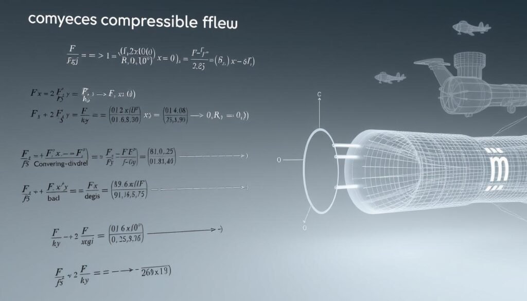
We share key equations for compressible flow used in aerospace and high-speed gas systems. These equations help with quick calculations of stagnation and static properties, shock behavior, and nozzle limits. They are essential for design and analysis.
Isentropic flow equations and Mach number relations
Pressure and temperature ratios are given by p0/p = (1 + (γ-1)/2 M^2)^(γ/(γ-1)) and T0/T = 1 + (γ-1)/2 M^2. Density ratios follow ρ0/ρ = (1 + (γ-1)/2 M^2)^(1/(γ-1)). Stagnation properties are values after reversible deceleration to zero velocity.
The critical state is at M = 1, a key point in many equations.
Normal and oblique shock relations
Normal-shock formulas give downstream Mach, pressure, and temperature from upstream M1 and γ. These are direct functions of M1. Oblique shocks require the shock angle β and flow deflection θ.
Engineers use θ–β–M charts or iterative relations to solve for post-shock conditions. Entropy rises across any shock, so post-shock stagnation pressure drops even when static pressure increases.
Nozzle flow and choked flow conditions
The critical pressure ratio for choking is p*/p0 = (2/(γ+1))^(γ/(γ-1)). When a nozzle reaches M = 1 at the throat, mass flow becomes independent of downstream pressure. ṁ = A p0/√T0 √(γ/R) (2/(γ+1))^{(γ+1)/(2(γ-1))}.
Area–Mach relations link cross-sectional area to Mach for isentropic nozzles. These guide contours in converging-diverging designs.
Practical notes and tools
Use gas property tables, NASA thermodynamic data, or computational tools for non-ideal or multi-component gases. Diagrams—nozzle Mach distribution and shock schematics—help visualize flow transitions and choked flow zones during sizing and performance checks.
- Quick reference: stagnation/static conversions and area–Mach relation for design iterations.
- Shock checks: compute entropy change and stagnation loss to assess performance penalties.
- Nozzle sizing: apply the choked mass flow equation early in preliminary design to set throat area.
Hydraulics and Pneumatics: System Design Equations

We have a set of useful formulas for designing hydraulic and pneumatic systems. This guide helps teams predict how well their systems will work. It also helps avoid common mistakes in design.
Hydraulic pump and motor power calculations
First, we calculate hydraulic power as P_h = Δp · Q. Here, Δp is the pressure rise and Q is the flow. To find the input power, we use P_input = P_h / η_p, where η_p is the pump’s efficiency.
For motors, we invert the formula and add mechanical efficiency. These formulas help size the prime movers correctly.
Pressure drop in pipes and fittings
The Darcy–Weisbach relation helps us find pressure drop: Δp = f (L/D) (ρV²/2) + ΣK (ρV²/2). We choose the friction factor f from the Moody chart or solve Colebrook for turbulent flow. For laminar flow, we use f = 64/Re.
These formulas help us pick the right pipe size and routing. They ensure the pressure at the actuator meets our needs.
Actuator sizing and flow control basics
For cylinders, force is F = pA. Pressure times area equals the static force. The flow needed to reach speed v is Q = A · v.
For rotary actuators, we convert torque to pressure and displacement. When designing valves, size them to limit pressure drop and avoid cavitation. These rules help in designing both hydraulic and pneumatic systems.
Pneumatics specifics
Air compressibility affects flow and force in pneumatic systems. We use formulas that correct for pressure, temperature, and compressibility. Regulators and flow control valves help stabilize speed and reduce shock.
Practical notes and safety
Use proper filtration and choose hydraulic oil by ISO grade. Fit pressure relief valves near pumps for safety. Always check your designs against industry standards.
- Check pump input power against motor ratings.
- Verify friction factor with Reynolds number and surface roughness.
- Confirm Q = A·v for each actuator motion cycle.
- Include regulators and accumulators for pneumatic circuits.
| Design Item | Key Formula | Typical Units |
|---|---|---|
| Pump Power | P_h = Δp · Q ; P_input = P_h/η_p | W, Pa, m³/s |
| Pipe Pressure Drop | Δp = f (L/D) ρV²/2 + ΣK ρV²/2 | Pa, m, m/s |
| Cylinder Force & Flow | F = pA ; Q = A·v | N, Pa, m², m³/s |
| Pneumatic Correction | Compressibility and regulator corrections applied to Q and p | Dimensionless, Pa, m³/s |
Instrumentations and Measurement Equations for Accuracy

We focus on the basics of measuring things accurately. This guide connects theory to real-world use. It explains how errors happen, how to mix different uncertainties, and how sensors turn physical signals into data. It’s a handy reference for mechanical engineering.
Error analysis is about separating two types of errors. Systematic errors cause a shift and need calibration. Random errors add noise and need statistical handling. For a model y = f(x1,x2…), use the formula σ_y = sqrt(Σ (∂f/∂xi)^2 σ_xi^2). The unit of σ_y matches the variable being measured.
Uncertainty propagation works best with small uncertainties. For correlated variables, include covariance terms: σ_y^2 = Σ (∂f/∂xi)(∂f/∂xj)Cov(xi,xj).
Calibration regression often uses a linear fit y = m x + b. Calculate the standard error of estimate and confidence intervals for slope and intercept. Use Python or MATLAB for this.
For regular checks, follow NIST standards and schedule calibrations. Temperature control and warm-up time reduce errors. Keep uncertainty budgets clear for calibration and drift.
Sensor equations vary by technology. Strain gauges use ΔR/R = GF·ε. Thermocouples follow standard polynomials and tables. Pressure transducers map pressure to voltage via sensitivity S (V/Pa).
We have a table comparing sensor relations, calibration needs, and units.
| Sensor Type | Primary Equation | Calibration Note |
|---|---|---|
| Strain gauge | ΔR/R = GF·ε ; V_out ≈ (V_exc/4)·GF·ε | Bridge balance, temperature compensation, NIST traceable standards |
| Thermocouple (Type K) | EMF = Σ a_n T^n (polynomial) ; use CJ compensation | Polynomial coefficients per ITS-90, cold-junction calibration |
| Pressure transducer | V_out = S·p + V_offset | Span and zero adjustments; sensitivity verified against dead-weight tester |
Practical tips: record raw data, propagate uncertainties, and store calibration outputs. We pair sensor equations with an error budget for quality decisions.
Tips for Remembering Formulas and Avoiding Common Mistakes

We share tips to help you remember formulas and avoid mistakes. Use short routines like review, label, and check to make formulas a part of your daily routine. These steps will boost your accuracy and confidence in design work.
Mnemonic strategies and formula grouping
Organize formulas by physical principle. This includes conservation laws, constitutive relations, and dimensionless groups. A mnemonic for grouping formulas makes it easier to recall during exams or design reviews. Try using SEED for Statics, Equilibrium, Energy, Dynamics and pair each with a sketch.
Flashcards and spaced-repetition apps are great tools. Create one card per principle with a short example. Regular review helps move formulas from short-term to long-term memory.
Dimensional analysis checks and unit consistency tips
Always check dimensions before accepting a result. Make sure both sides of an equation have the same units. Convert US customary units to SI early to avoid errors.
Keep track of significant figures based on input precision. Use dimensional shortcuts to spot mistakes quickly. These tips save time and catch errors.
Common sign, sign convention, and algebra pitfalls
Choose a consistent positive direction for free-body diagrams. Label moments and forces clearly to avoid sign errors. Mistakes often come from inconsistent signs or swapping plus and minus.
Be careful with roots, powers, and superposition steps. Squaring or taking square roots can introduce errors. Peer review critical calculations to avoid mistakes.
Practical checklist
- Make a personal quick-reference index of frequently used formulas and test each with a short example.
- Use visual mind maps to link related equations; the visual cue acts as a memory anchor.
- Validate with dimensional checks, then cross-check results using an alternative method when possible.
- Ask a colleague to review high-stakes calculations to further reduce the chance to avoid engineering mistakes.
Adopt these habits to make formulas reliable tools. With practice, mnemonic techniques, and dimensional analysis, we build systems that catch errors before they affect the design.
Downloadable Resources: PDF Cheat Sheet and Printable Reference
We offer a downloadable PDF cheat sheet. It’s a two-page quick reference for mechanical engineering formulas and units. You can also get an editable spreadsheet and LaTeX source for customizing.
The PDF is 20–40 pages long. It’s a detailed handbook with clear explanations, examples, diagrams, and tables. It follows NIST, ASME, and AGMA standards. You can search the text and find cross-references for study and design checks.
Files are free for educational use. They include a unit conversion chart, an equation checklist, and blank free-body diagram sheets. You can also get LaTeX sources and an editable spreadsheet for teaching or CAD.
This resource is always improving. Download the handbook and cheat sheet. Use the formula sheet on the job. Share your feedback to help us improve. Subscribe for updates and example problems.


Leave a Reply